

Can one improvement help a model discover the next?
A model that becomes better at finding useful edits could help produce its next improvement. That is the recursive self-improvement loop we want to test. Astra’s edit of Qwen gives us a concrete place to start: a steering rule stored in the weights, whose push changes with the model’s state.
In the Weight-Space Programming study, Astra changed selected columns in two MLP matrices. Takehi and colleagues reported that MATH-500 accuracy rose from 7.9% to 48.1%, while the fraction of answers hitting the token limit fell from 93.0% to 33.1%. Gradient-based training was not allowed. Those benchmark results belong to the original authors; our experiments examine the mechanism of the released edit.1
Our contribution is to connect the rule Astra wrote, the corrections shared weights can express, and the output changes Fisher geometry predicts locally. We reconstruct the edit as activation steering and measure where the geometric prediction holds. The underlying algebra is established; applying it to this released edit gives us concrete questions to test next.
For an engineer, the suggested workflow is straightforward: try a correction in activations, check whether the permitted weights can implement it across inputs, then evaluate the edited model. Geometry describes the reachable corrections and gives small changes in the output distribution a common measure. Along the tested direction, Fisher predicted small changes well and lost accuracy at the original edit strength. Whether it helps us choose better edits is the next experiment.
The repair itself began with 85 unfinished answers.
When Astra asked Qwen3.5-0.8B to solve 96 practice problems, eleven answers were correct. The other 85 ran through the 32,768-token budget without reaching an answer. Their final passages repeated the same phrases over and over. Before any geometric analysis, Astra already had a useful lead: a recognizable pattern of failure.3
How did an LLM find where—and in which direction—to intervene among hundreds of millions of parameters?
A trained network gives us places to observe internal features and change their effects. We can measure activations, modify the matrices that write them into the residual stream—the representation successive layers read and update—and check the output. Astra used this structure to find a compact edit, with a different direction at each edited layer. Once stored, the rule reads the current activations and scales its correction accordingly.
We will follow the failure Astra observed, the program it wrote into the weights, and the geometry of that program’s effects. Then we will ask how this could become a repeatable method across models, and whether a successful edit could help a model become better at making the next one.
Experiment inventory and scope
What the evidence covers. The large benchmark improvement comes from the original authors. Our experiments comprise a reconstruction on 40 prefixes, local-KL measurements on 32 prefixes, and a steering-control experiment using artificially repetitive text. A prefix is the sequence of preceding tokens supplied to the model. A small generation pilot is complete; full MATH-500 reproduction and the fixed-program search study remain unfinished. The paintings are allegories. The mathematical surfaces come from explicitly defined models.
Astra did not need to understand the meaning of every weight. It found a measurable failure and a linear projection where a short rule could act on it. The edit reads a scalar from incoming activations and adds a correction along a fixed direction. This raises two questions: can one shared matrix produce the corrections we want, and how much do those corrections change the output distribution? The first concerns a reachable subspace; the second concerns a metric.
The division of labor is important. The logs provide evidence about how Astra discovered the failure and selected an edit. The algebra explains how the stored edit executes once it has been found. Fisher geometry supplies a local, prospective description of output change and reachability; it does not explain why Astra discovered this particular direction or why it chose these layers and gain.
1. What could Astra observe?
Start with the task and the tools. The initial prompt gave Astra Qwen's architecture, functions for reading and writing weights, labeled practice problems, and tools for collecting outputs and activations. It even named repetition as an example of a failure worth repairing. Astra was asked to classify failures, test interventions rather than stop at correlations, vary their strength, and check the results on unused questions.2
The run with a budget of 50 evaluation-tool calls could repeat this cycle of observation and intervention. Here, “50” counts tool calls, not model forward passes: one call could run hundreds of generations or evaluate supplied text under teacher forcing, where supplied tokens rather than sampled tokens determine each next-token evaluation. Astra inspected answers, measured internal quantities, tried edits, and used behavior on held-out questions to decide what to try next.
The logs preserve failed requests and inconclusive early results. A single-neuron ablation and a subsequent removal of a direction in one layer each produced a noisy +6.25 percentage-point change on 32 problems. A later edit to layers 15 and 19 together produced a much larger held-out improvement. The repair emerged through this sequence of trials.
Three features of the setup made the search tractable. First, the failure was visible: many answers followed the same pattern of prolonged repetition ending at the token limit. Second, access to activations and log-probabilities made it possible to compare repetitive and non-repetitive text quantitatively. Third, the MLP down-projection provided a linear path for writing into the residual stream. This structure made a short corrective program possible. The results alone do not tell us how much of the success came from Astra's reasoning, the prompt, the tools, or a failure that happened to be amenable to this kind of repair.
The shorter 10-call and 25-call runs identified the same broad failure but produced less effective edits: a weaker rank-one-style operation across many output matrices, and an attention-head ablation. The same diagnosis did not guarantee the same solution.
The public logs report three contrasting runs. All three are the original authors' results, not our reruns.
| Reported run | Evaluation budget | Edit described in the released brief | Reported MATH-500 accuracy |
|---|---|---|---|
| p10c | 10 evaluation API calls | Remove a loop direction from 30 matrices across layers 8–22, gain 1.5 | 12.3% |
| p25c | 25 evaluation API calls | Disable head 7 in layer 15 | 14.1% |
| p50c | 50 evaluation API calls | Subtract a masked direction in 64 columns per layer, MLP layers 15 and 19, gain 6 | 48.1% |
The table compares the programs each run actually produced. Evaluation budget measures resources; it does not by itself establish why the scores differ. The original README also reports the unedited accuracy of 7.9% and the changes in truncation rate. The 48.1% result, like the other entries, is an original report rather than an independent full reproduction here.1
It would also be premature to conclude that the edit gave Qwen new mathematical abilities. Although the evaluation used mathematics problems, the observed bottleneck was finishing an answer. On the original confirmation set, the edited model completed many answers that had previously exhausted the token budget. Correct answers after editing were longer, rather than merely ending sooner. That pattern is consistent with removing repetition that prevented existing competence from producing an answer. It does not establish that a low-rank intervention added general arithmetic or algebraic ability.
Evaluation should preserve that distinction. Alongside overall accuracy, we should count answers rescued by the edit, previously correct answers lost, completed but incorrect answers, answer lengths, and degeneration into repeated whitespace.
The practical lesson is to make the failure measurable before choosing an edit family. An aggregate score cannot tell us whether errors share an internal state, reflect a missing feature, arise from decoding, or have unrelated causes. The 85/96 observation narrowed the search before a geometric interpretation was needed.
2. How does a 0.016% edit act as a program?
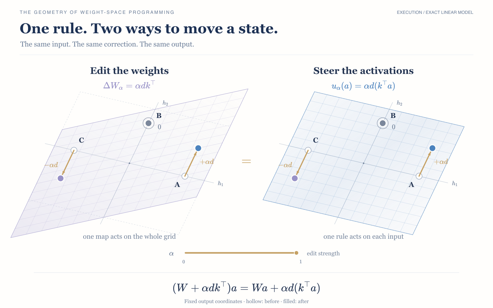
One shared matrix applies a different correction to each input. At a linear projection, a weight edit and an activation hook implement the same rule exactly. This is a mathematical example.
View full size ↗Settings, scope and source files

One edited matrix can move different inputs by different amounts—even in opposite directions. The figure shows that same rule executed in two ways: stored in the weights on the left, and applied to the activations on the right. Corresponding outputs coincide.
How to read the linear example
The figure uses a precisely defined toy model to compare two operations. It is not a recording of Qwen activations. Take three states, A=(1,0), B=(0,1), and C=(-1,0), with W=I, k=(1,0), and d=(0,.7). On the left, one edited matrix transforms an entire grid of inputs. On the right, the same correction is applied separately to each activation. Both are drawn in fixed output coordinates: hollow points mark original outputs and filled points mark edited ones. At full strength, A moves by +d, B stays still, and C moves by −d.
The animation gradually increases the edit strength in both panels. Corresponding points coincide throughout. This illustrates an algebraic identity, not Astra’s search or measured Qwen dynamics. A single external push on A would not, by itself, specify a policy for later inputs.
The actual edit acts on the MLP down-projections in layers 15 and 19. Let map MLP-neuron activations into the residual stream. The mechanism follows from an exact identity:
The 0.016% figure is an approximate parameter-count ratio: 131,072 targeted entries (2×64×1024) out of roughly 800 million model parameters. It is not a relative weight norm or the fraction of the two MLPs. Read a scalar from the current state, multiply a direction vector by it, and add the result to the activations. The scalar varies continuously and can be positive or negative. Calling it a “gate” does not make it a binary loop detector. Astra's idealized edit at each layer takes the form
where is a unit direction, is a mask selecting columns, and is the gain controlling intervention strength. The resulting activation change is
The vector determines which direction to move. The scalar multiplying it depends on the current MLP activations and determines when and how strongly to move. The weights therefore store a state-dependent steering rule, rather than an instruction to add the same vector every time.
At a linear projection, the possible interventions can be organized as follows:
- Add a constant vector, also achievable with an editable bias: .
- Read one scalar and use it to scale a direction: .
- Assign an output vector to each neuron: .
- Specify an arbitrary change for each input: .
This is a classification of interventions at a linear interface, not a theorem about minimizing KL. A bias-free matrix, for example, cannot necessarily add the same nonzero shift to every possible input; an editable bias makes that operation available. Nor can a single shared matrix generally implement an arbitrary field of changes. Its Jacobian determines which changes are reachable.
In the actual edit, each of the two layers has its own direction and 64 selected columns. The published formula remains rank one after masking, before rounding to bfloat16. The saved weight difference also contains small rounding residuals. The original evaluation used those saved weights; the ideal formula explains the mechanism. Keeping the two distinct matters for reconstruction.
In E1, we compared the saved weight edit with its additive activation intervention on fixed prefixes. Across 40 prefixes in FP32, the maximum logit difference was , and the maximum KL was . Differences were larger in bfloat16: a maximum logit difference of 0.3047 and maximum KL of 0.00713. This experiment checks numerical reconstruction of the edit. It does not provide a new task-performance result.
The gain matters to the interpretation. A gain of one removes the selected columns' component along . A gain of six changes that component to approximately negative five times its original value, reversing it rather than merely removing it. Where the selected neurons write along the contrast direction, the edit adds a contribution in the opposite direction. Calling this only an “ablation” obscures the feedback-like behavior. It still does not establish that the gate selectively detects every naturally occurring loop.
With edits at multiple layers, the activations used by each intervention matter too. Layer 19 receives inputs already affected by the edit at layer 15. The additive identity remains exact when comes from the edited execution. Replaying gate values recorded from the unedited model does not exactly reproduce the edited model. The switch must be evaluated from the activations that arrive at that moment.
When the weight edit and activation hook agree
For one linear projection, arrange the neuron activations for each sample in rows:
# W: [residual_dim, neuron_dim]; u: unit direction
readout = mask * (u @ W)
D = -gain * u[:, None] * readout[None, :]
edited_write = a @ (W + D).T
hooked_write = a @ W.T + a @ D.T
The two expressions agree in exact arithmetic. To reconstruct the released model, use the actual saved difference , including its rounding residuals. At each later edited layer, use activations that already reflect the earlier interventions.
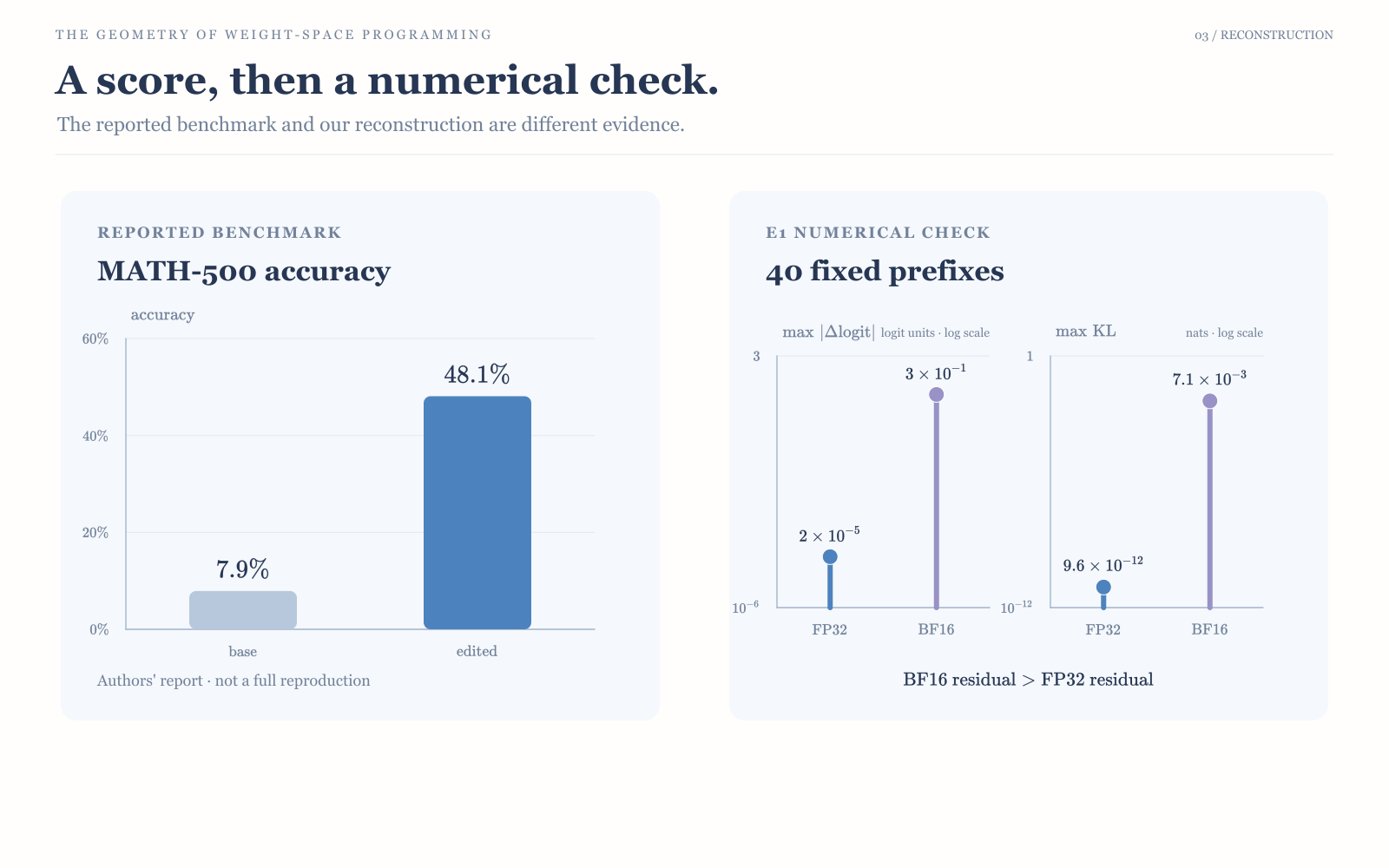
The benchmark improvement is the original authors’ result. Our E1 instead checks numerical agreement between a weight edit and an activation hook on 40 fixed prefixes; it does not repeat the full benchmark.
View full size ↗Settings, scope and source files
We also completed a small generation pilot. On eight selected problems, we generated one sample per problem from the unedited model and four from the edited model. The respective correct counts were 0/8 and 8/32; truncation counts were 8/8 and 18/32. This pilot checked the generation pipeline and measured runtime. Because sampling counts differ between conditions, it is not a matched estimate of performance on the full benchmark.4
Changing scales the arrow ; negative values reverse it.A gate is a signed command
3. Did the switch need to depend on the state?
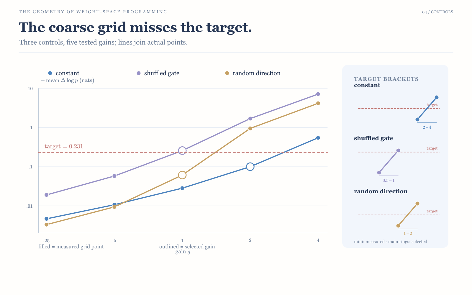
All three controls bracket the target but miss it at the selected gains. Without matched effects, this synthetic teacher-forced comparison cannot establish whether the gate is necessary.
View full size ↗Settings, scope and source files
To test whether the state-dependent switch matters, replace it with a constant intervention along . If the two have the same effect on repetitive text, which better preserves text associated with useful output? The preregistered E2 comparison included Astra's original gate, a constant intervention, shuffled gate values, and a random control. Two limitations constrain what the measurements can tell us.
First, the repetition was constructed. The E2 manifest explicitly describes a test using synthetic continuations under teacher forcing, rather than repetition generated by the model. It uses 16 calibration cases and 32 evaluation cases. Repetitive text is made by taking a reference-answer prefix and repeating its final 16-token block. Qwen did not enter these loops during generation. The experiment probes the edit's response to a controlled state; it does not directly reproduce the failure Astra observed.
Second, the effects were not successfully matched. The constant, shuffled, and random conditions all failed the predeclared effect-matching check. Their calibration residuals relative to the target were +0.1312, −0.0266, and +0.1701, respectively. With effects unmatched on the tested gain grid, we cannot make a clean comparison of side effects at equal benefit.
The results are still informative about response patterns. The original gate responds differently from the controls, and we can compare responses at teacher-forced positions in productive and repetitive sequences. But this does not show that thermostat-like, state-dependent control is necessary during natural generation.
All three calibration curves bracket the target, so a finer gain search may improve the match. The next experiment should keep the same controls, refine that search, and construct contrast pairs from answers the model actually generates on practice problems. Calibration and evaluation data must remain separate, and matching the target effect must be a prerequisite for comparison. We can then ask how the controls change the probability of entering or escaping a loop during generation, beyond their effect on the log-probability of a synthetic continuation.
4. How far can Fisher geometry predict the effect?
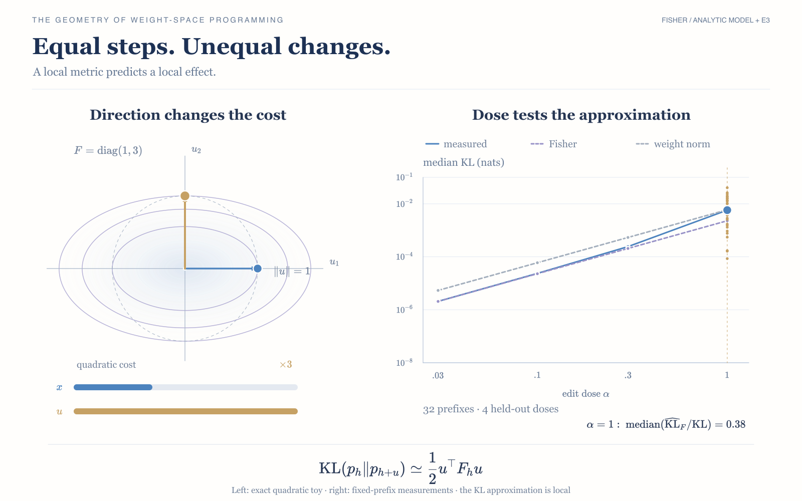
Equal-length moves can have different local costs (left: mathematical example). In E3 (right), Fisher predicts small KL changes well but loses accuracy at the original edit strength.
View full size ↗Settings, scope and source files

A norm measured directly in weight coordinates can be a poor guide to an edit's effect. Two weight changes of the same size can change the output distribution by very different amounts. For a fixed prefix and a small activation displacement , the next-token KL has the local expansion
where is the output Fisher matrix pulled back to activation coordinates. This metric measures how distinguishable the distributions are. It does not measure whether an answer is correct or its meaning is preserved. A low-KL intervention can still damage an unmeasured capability. Keeping KL low on text associated with useful output is a design objective we choose, not a guarantee supplied by Fisher geometry.
E3 tested this prediction on 32 evaluation prefixes. We estimated Fisher separately for each prefix using finite differences, and fitted the scalar coefficients of the norm baselines on 16 separate calibration prefixes. The evaluation strengths—0.03, 0.1, 0.3, and 1.0—were excluded from the local fit.
At strength 0.03, the median absolute prediction error on a log scale was 0.013 decades for Fisher, compared with 0.479 for the weight-norm baseline. At strength 1, the errors were 0.462 and 0.420, respectively. By this measure, Fisher was substantially more accurate for the small intervention, but slightly worse at the original edit strength.
At full strength, the median ratio of the Fisher prediction to measured KL, computed separately for each prefix, was about 0.38. This is the median of those ratios, not the ratio of the two medians. Agreement at the small strengths used to estimate or check derivatives cannot be counted as independent evidence of predictive accuracy.
Strength 1 corresponds to Astra's gain-six edit. At the strength that improved the original task, the local Fisher approximation was no longer accurate. Task improvement therefore does not validate the local approximation: an edit can leave the local regime and still help. The metric describes nearby changes; it does not automatically describe an entire generation.
These measurements also condition on a fixed prefix. During generation, changing the next token changes subsequent prefixes and their Fisher matrices. A theory of the whole sequence would need to specify both the sequence distribution and the intervention path. The fixed-prefix result cannot simply be extended to the entire rollout. Our theory note keeps these questions separate and leaves guarantees over finite trajectories as an open extension.
Conditions of the local-KL experiment
We computed KL in FP32 using ordinary softmax distributions at fixed prefixes. The calculation excludes the top-k and top-p truncation used during generation. The primary finite-difference step was 0.001; steps of 0.003 and 0.01 were used to check the derivative estimate. Only one saved edit direction was tested.
The activation-norm baseline uses activations from the intervened execution, so it is not a prediction available from the unedited state alone. This experiment also does not establish that a Fisher estimate transfers to another direction or another prefix.
5. What can one matrix do—and what changes with the metric?
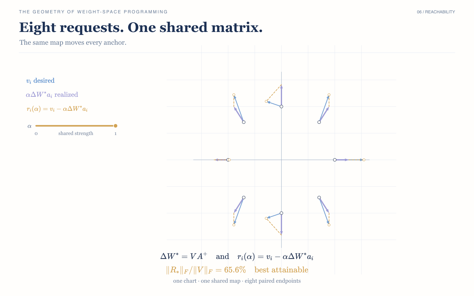
Eight requested changes must share one matrix. In this constructed example, even the best fit leaves a residual: the matrix cannot move every input independently.
View full size ↗Settings, scope and source files

The figure puts the requested and realizable changes on one coordinate chart. At each of eight inputs, a blue arrow shows the requested change and a violet arrow the change produced by the shared matrix. All eight violet arrows depend on the same matrix, so they cannot be adjusted independently. Gold segments join the two endpoints: they are the part of each request that the matrix does not realize.
Eight-input toy setup and least-squares diagnostics
Put the eight inputs in the columns of and their desired activation shifts in the columns of . One 2×2 matrix update must fit all of them. If we measure error with the Euclidean metric , the least-squares solution is
The animation varies the update from zero to this solution. All eight arrows move together, while the gold segments connect their endpoints to the requested endpoints. Even at the optimum, the residual's Frobenius norm is 65.6% of the norm of the desired field.
That number comes from this constructed example, not from Qwen. The animation interpolates toward a solution we have already computed; it does not record Astra's search or the steps of an optimizer.
The model file contains the inputs, requested changes, solution, and residual. The normal-equation residual is about . The remaining error is nonzero, but orthogonal to the space of realizable changes. What happens to the closest solution if we change the metric?
Which change is closest?
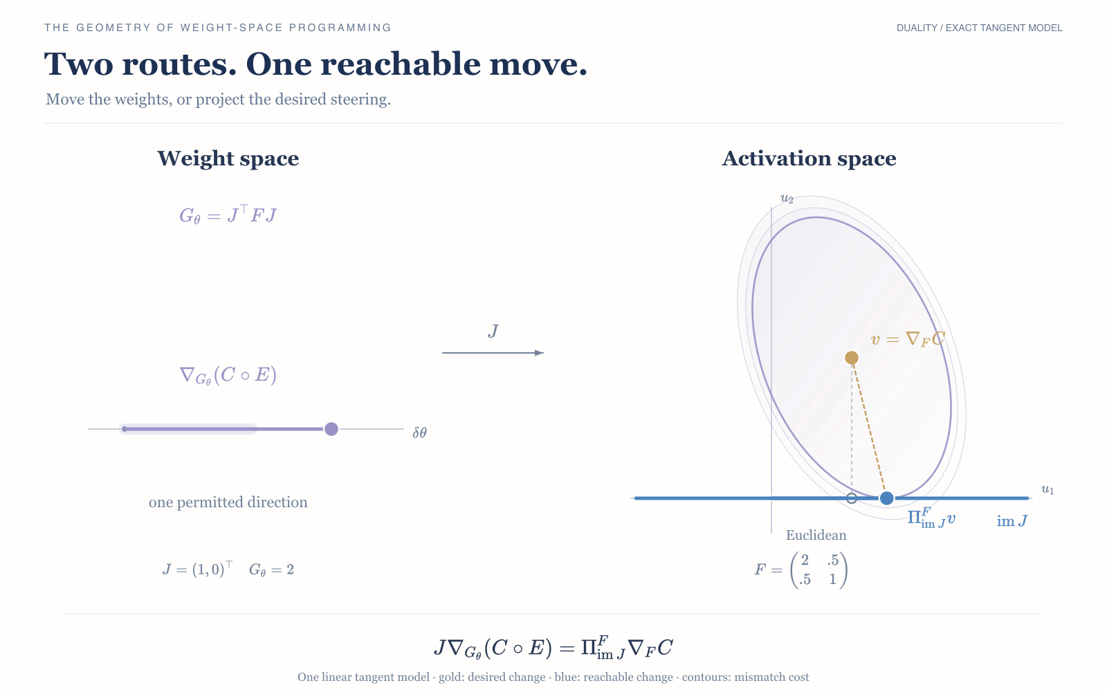
With a complete interface and its pulled-back Fisher metric, the two routes agree locally: move the weights along their natural gradient, or project the activation natural gradient onto reachable changes.
View full size ↗Settings, scope and source files

The right panel shows the desired activation change and the line of changes that the permitted weight edits can realize. The ellipses measure mismatch from the desired change. Shrinking an ellipse until it touches the line identifies the closest reachable change in the Fisher metric; the open gray point marks the different Euclidean projection. On the left, a natural-gradient step in weight space maps to that same reachable change. The synchronized arrows show the two routes to one result.
The operational question is simple: if several inputs request different changes, how much of that field can one shared matrix realize, and which realizable change is least costly? The figure makes the first constraint visible; the formal conditions are in the foldout.
The weight-to-activation relation is an adjoint and metric relationship. Let map the permitted weight coordinates to the state at the intervention interface, with derivative . This state may collect activations across many inputs. With the downstream computation held fixed, it must capture every effect of the weight edit on that computation. This is the requirement for a complete intervention interface.
Pulling the activation-space metric back through gives the weight-space metric .
A natural gradient gives a direction for changing an objective, with distance measured by the chosen metric. We label that metric below the gradient symbol. The equation says that two ways of choosing a feasible activation change agree:
In identifiable coordinates, or on the quotient by null directions described below, a smooth objective satisfies The left-hand side is the activation change induced by moving the weights along their natural gradient. The right-hand side projects the activation-space natural gradient onto the changes those weights can realize, using the Fisher metric. Locally, taking a natural-gradient step in weight space and mapping it to activations gives the same result as taking the natural gradient in activation space and projecting it onto the reachable directions.
Metric-gradient definition and the shared-input metric
To specify which metric defines the gradient, we use the metric-gradient operator . It converts the differential of a scalar objective into a direction using the metric . For positive-definite and every tangent vector , it satisfies Here is the first-order change in along , and collects the ordinary coordinate derivatives in a column. Setting recovers the Euclidean gradient; using a Fisher metric gives the natural gradient. The subscript specifies the metric, not the direction of differentiation. This operation raises the differential's index with the inverse metric. It is distinct from taking the covariant derivative of a vector field.
For a single linear write projection, , and averaging the pullback metric over inputs gives . Every input in that average uses the same parameter update. Steering one input therefore cannot be chosen independently of the effects on the others.
The projection identity: proof and conditions
In differential-geometric index notation, where denotes the inverse metric and repeated indices are summed. The covariant derivative of a scalar satisfies ; raising its index gives the gradient vector. Our subscript is a metric label, whereas the index in denotes a coordinate direction.
Assume is positive definite on identifiable activation coordinates. Write for the coordinate representation of the differential . If is singular, interpret its gradient on the quotient by . Choosing the Moore–Penrose representative, which minimizes Euclidean norm in the chosen weight coordinates, gives The -orthogonal projector is . Applying it to gives the same expression.
If the Fisher metric itself is singular, work on an identifiable quotient space and require the objective differential to vanish on null directions. Simply substituting a Euclidean pseudoinverse does not make the statement coordinate-invariant.
The downstream map must remain fixed. For interventions at multiple sites, account for their dependencies through a complete interface or an explicit intervention graph. The identity establishes local agreement; it does not imply that optimization trajectories coincide after finite steps.
Amari preview and vector-covector distinction
The second is Amari's duality between natural and expectation coordinates, which appears when the output is represented by an exponential family. If denotes softmax natural coordinates and the expected sufficient statistics, then
A straight path in expectation coordinates generally becomes a curve in natural coordinates, and vice versa. This provides a mathematical basis for “dual steering” at the output representation. It does not make the weights themselves expectation coordinates, or make every hidden layer dually flat. Nonlinear intermediate computation, rank deficiency, and unidentifiable directions each require their own conditions.
Together, these relations give us a mathematical account of the Qwen edit: a rank-one update can apply a direction with input-dependent strength, and a Fisher-weighted alternative could reduce output KL while preserving a fixed local target effect. They do not explain how Astra chose its contrast examples, why the two layers looked promising, or why it tried gain six. The logs show a search that adapted to observations, not evidence that these choices came from a Fisher calculation.
It is important here to distinguish a vector from a covector. An activation difference between two classes of text is a displacement vector: it describes how the representation changes. The differential of a behavioral objective is a covector: it measures how much that objective changes under a small displacement. Using the Fisher metric to relate them requires specifying the metric and a local output model.
Replacing every contrast vector with does not automatically produce natural-gradient steering; it confuses two different mathematical objects. The proposed E5 experiment specifies the objective, the positions at which cost is measured, damping, and the effect-matching procedure in advance. Its candidate direction is defined under those conditions, rather than by a general prescription to precondition every useful direction.
The phrase “compiled into weights” carries the same constraints. It means that an editable matrix implements a particular field of activation changes across a set of inputs. The resulting program need not be independent of those inputs, cannot generally implement arbitrary fields, and is not guaranteed to preserve every other function. A shared matrix links its effects across contexts. Even a successful edit is one choice from a constrained family of functions, and its side effects are part of what that program does.
For edit design, this suggests an order of work. First check which requested changes the permitted weights can produce. Then compare feasible changes using a cost defined on the outputs we want to preserve. A metric can help choose among them; whether the resulting edit helps during generation still needs a separate test.
Can we get the same effect at lower cost?
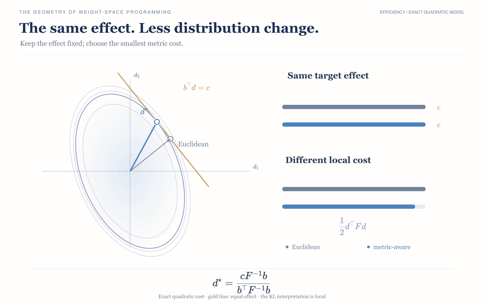
Keep the first-order target effect fixed, then find the change with the smallest quadratic cost. The geometry gives an optimal candidate in this model, not a demonstrated improvement to Qwen.
View full size ↗Settings, scope and source files

Every point on the gold line in this figure produces the same target effect to first order. The ellipses show a quadratic cost for changing the output distribution we want to protect. Moving along the line toward the smallest ellipse that touches it preserves the target effect while reducing that cost. The blue point is the least costly change. The paired bars make the comparison explicit: the effect stays fixed while the cost falls.
For a positive-definite metric , nonzero objective differential , and target effect , the optimal displacement is
The figure uses an explicitly defined two-dimensional quadratic model. The points represent equal-effect candidates, not measurements of Astra's edit. The animation moves among those candidates to explain the geometry; it does not replay the search.
To use this idea in a real editing experiment, we would need to estimate the metric, match the target effect, and evaluate behavior on held-out data. Information geometry provides a candidate direction and a way to compare it with alternatives. That role does not imply that Astra's earlier search was a natural-gradient algorithm.
Minimum cost at a fixed target effect
Minimize subject to . The stationarity condition gives , and substituting the constraint yields the solution above. Write any other feasible point as . Then , so
This result is exact for the quadratic form. Interpreting it as a KL cost requires a local approximation. The metric can be defined in activation coordinates or in the permitted weight coordinates, related by the pullback . The rank and null-direction conditions above still apply.
6. Why do shared weights make some steering requests impossible?
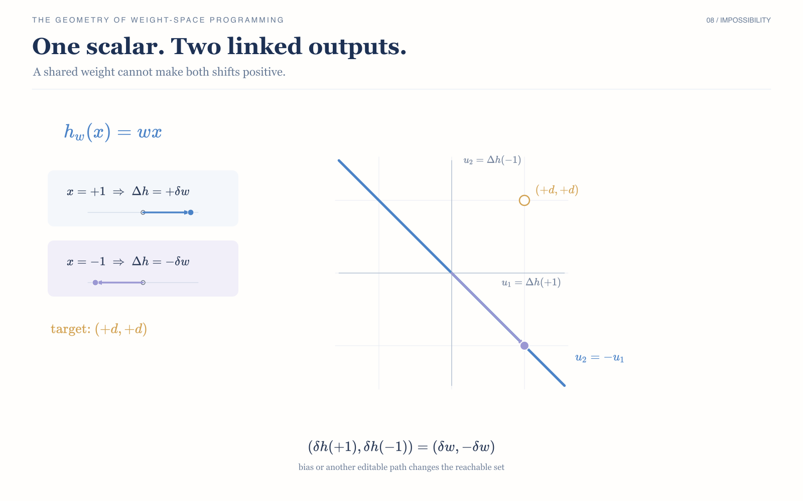
One weight moves the two inputs in opposite directions, so it cannot shift both positively. This exact counterexample assumes a bias-free linear model; an editable bias changes what is possible.
View full size ↗Settings, scope and source files

Consider a model with just one weight, , evaluated at and . Changing the weight by shifts the two activations by and . The shifts necessarily point in opposite directions.
Now suppose we want the same positive shift for both inputs. Direct activation steering can add . A shared weight edit would have to satisfy both and , which is impossible for .
This small example exposes the constraint. A weight edit cannot specify an independent intervention for every input: the same parameter change links all of its effects. More generally, consider the local linearization, in which maps permitted weight displacements to activation displacements. Within this linearized model, only changes in are reachable. For a reachable change , with a positive-definite metric measuring resource cost in weight space, the minimum cost is
If the requested change lies outside , no edit satisfies the constraint, and the cost is . Evaluating the pseudoinverse expression alone must not be used to assign a finite cost to an unreachable request. These feasibility and cost statements are exact for a linear interface. For a nonlinear model, an infeasible linearized request does not by itself rule out a finite edit. Dual variables can certify infeasibility in the linearized model. Such a certificate can guide a practical decision: add a bias, edit another layer, relax a constraint on a protected context, or stop searching.
Fisher alone also cannot select a sparse edit. Different weight changes can induce the same local activation field and therefore have the same output Fisher cost. Choosing 64 columns, two layers, or a particular sparse mask requires an additional resource constraint, architectural prior, or search rule. Astra's mask was observed as part of a successful program; the metric does not determine it uniquely.
7. Where does Amari's duality enter?
We can now visualize the other duality: the relationship between natural and expectation coordinates.
Take a three-class softmax and remove the redundancy by fixing the third logit at zero. The remaining two logits are natural coordinates . Define Expectation coordinates give the probabilities themselves; natural coordinates give the log-odds . These are different coordinates for the same distribution. Since the Hessian of is the Fisher matrix, Moving at constant velocity in expectation coordinates generally requires the velocity in natural coordinates to vary. The animation shows the same evolving distribution in both coordinate systems.
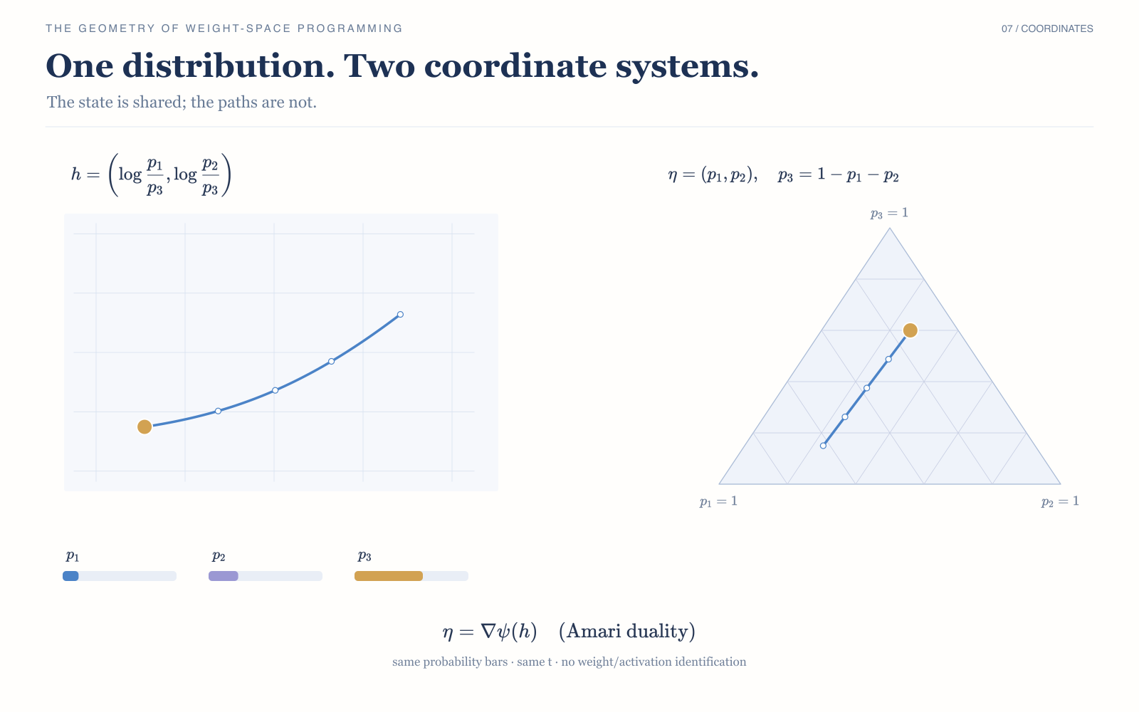
A straight path in probabilities generally curves in log-odds. Both panels describe the same changing distribution. This softmax coordinate duality is distinct from the relationship between weights and activations.
View full size ↗Settings, scope and source files

The coordinate transformation is computed analytically; it is not a landscape measured inside Qwen. One view uses log-odds, while the other uses the probability simplex. The synchronized bars make it clear that the two paths, despite their different shapes, represent the same probabilities. On the interior of the simplex, the dual potential is negative entropy, .
This duality must be distinguished from the weight-to-activation projection identity. Weights and hidden activations are not automatically each other's Legendre-dual coordinates. An arbitrary intermediate layer need not form a minimal exponential family or a dually flat space.
We can pull the output metric back to a hidden layer. That alone does not give the layer a globally dually flat structure.
Even so, once we specify a behavioral objective, the geometry suggests a concrete edit to test. Let the covector measure the desired first-order change, and let measure cost on contexts whose useful outputs we want to preserve. A damped candidate direction is proportional to . Whether it helps must be tested at a matched target effect. This remains a research proposal; it has not been shown to improve on Astra's edit.
8. What can we build from this?
Astra found a small program that runs inside Qwen. The edit reads the current activations and changes how the model writes into its residual stream. The public logs show how Astra moved from a recurring failure through contrast measurements, interventions and gain sweeps to improvements on held-out questions.
Our contribution is to make that program something we can reconstruct and reason about when designing another edit. The exact linear identity connects weight changes to activation interventions. The shared-weight constraint tells us which corrections can coexist across inputs. Fisher supplies a local measure of their effect on the output distribution. Together, these let us test a correction, check whether it can be stored in the permitted weights, and compare changes to behavior we want to preserve.
Our E1 experiment reconstructed the edit as an additive intervention and confirmed numerical agreement in FP32. E3 found that Fisher geometry predicted small KL changes at fixed prefixes well, but the prediction broke down at the original gain-six strength. That result locates the limit of the approximation; the original edit still improved the reported task results. E2 measured responses to constructed sequences. Because those sequences did not arise from natural generation and the control effects were not matched, it cannot establish whether the switch is necessary during generation.
Those results suggest the following workflow for the next experiment. It combines checks we have performed with comparisons still to be run.
| Decision | Evidence-led action | What it establishes |
|---|---|---|
| Diagnose a recurring failure | Measure completion, repetition, truncation, and internal contrasts before editing weights. | Whether a shared, measurable bottleneck is a plausible target. |
| Prototype an activation hook | Implement the candidate correction at the MLP down-projection and inspect its state-dependent response. | Whether the proposed rank-one rule can be reproduced numerically. |
| Match controls | Tune constant, shuffled, and random controls to the same target effect before comparing side effects. | Whether a claimed benefit survives equal-effect comparison. |
| Sweep intervention strength | Measure local and larger strengths separately, including the full-dose setting. | Where a local metric is predictive and where it stops being so. |
| Test shared constraints | Fit requested changes across inputs and inspect residuals and reachability. | Whether one shared weight matrix can express the proposed steering field. |
| Validate held-out generation | Evaluate naturally generated, held-out trajectories and task outcomes with matched sampling. | Whether a fixed-prefix or teacher-forced result transfers to generation. |
From a working correction to a reusable method
The same algebra applies wherever an editable linear map writes into a model’s activations. Useful directions, gates and intervention sites may differ, but the design questions carry across models: find a useful steering rule, check which part shared weights can implement, and test the stored rule on new inputs. Independent WSP follow-up experiments report gains on several tasks, alongside uneven transfer and searches that retained the original model. The next opportunity is to make discovery reliable.
This connects directly to current work on model control. Anthropic's Assistant Axis uses activation constraints to stabilize behavior. Goodfire's manifold steering studies interventions that follow the geometry of representations. Our complementary question is which of those useful interventions a shared weight edit could implement. The projection identity gives that question a precise local form. Some requested corrections lie outside the reachable space; identifying them helps us decide when to change the edit family or keep an intervention in activation space.
To test the practical value of geometry, we would preregister a comparison against simpler editing choices, keeping the original behavioral target fixed. Match the target benefit and total budget, including the cost of estimating the metric, then compare behavior on held-out tasks. Use naturally generated trajectories alongside synthetic controls, and keep discovery data separate from evaluation data. Controls that preserve intervention magnitude while disrupting the proposed mechanism would help identify what makes a correction work.
This experiment asks whether the metric can help us predict which edits preserve more of the behavior we want before we spend heavily on generation. Its outcome would determine how useful geometry is for choosing edits. The original logs already provide a working example of an LLM finding a compact rule through observation, internal measurements and iterative tests.
Can an improvement help produce the next one?
The exciting possibility is that an edit makes a model better at finding its next improvement. A repair that lets an existing ability work more reliably could also help the model propose or assess better edits. Astra was the editor and Qwen the target in the case studied here. Improving the editor’s ability, and sustaining that improvement over rounds, are the experiments we now want to run.
Start by comparing edited and unedited models as editors of the same frozen target checkpoints. Give them the same tools, evidence, feedback and compute budget. Then compare an editor that changes across rounds with a fixed editor given the same accumulated history and total budget. In the recursive condition, each accepted edited checkpoint takes over as the editor for the next round. Re-estimate activations and the local metric after each accepted edit.
Keep the tests used to accept an edit separate from a sealed final evaluation. Count failed searches as well as successes, and evaluate successive rounds independently. This would let us ask whether improving the editor improves the edits that follow, and whether that effect lasts. The Astra–Qwen run supplies the starting point; it has not demonstrated this feedback loop.
That question connects WSP to the wider effort to automate AI research. OpenAI’s account of research acceleration and METR’s assessment at Anthropic examine how AI contributes to further model development. WSP offers an operation whose effects we can inspect: a model proposes a weight change, we examine what it does, and independent evaluation decides whether to retain it. Our proposal is to use geometry to help design and test these operations, then ask whether the models become better at the process itself.
Scope, unresolved questions and prior work
Here, “one model and one failure mode” refers to the Astra–Qwen case analyzed in this essay. It does not describe the full range of experiments in the original WSP report, and this case alone cannot establish how WSP scales in general. There is no evidence that Astra used Fisher geometry. Nor have we shown that gated rank-one instructions are generally easy to discover. We have not established whether the edit added an ability or removed an obstacle to an ability the model already had.
Information geometry guides experiments and helps identify impossible requests; it does not replace diagnosis or behavioral validation. The generality of the linear identity gives us a common mathematical framework across compatible model interfaces. Whether useful edits can be found reliably across model families, and whether improvements persist over successive rounds, are empirical questions.
These connections build on prior work: Amari's natural gradient, Steer2Edit, and FishBack. This essay tests their scope in one WSP case; it does not claim the dualities are new. Its contribution is the connection between the released program, numerical reconstruction, local geometry and a procedure for testing future edits.
Astra’s edit gives us a useful rule to inspect, execute and test. The opportunity is to turn that understanding into a reliable method across models—and to test whether one improvement helps a model discover the next. That is a concrete research goal for connecting model control to recursive self-improvement.
Appendix. Where do LoRA, model synthesis and Model Map fit?
The Qwen case gives us a rule we can inspect. Three connections help us ask what carries beyond that case: how a learned LoRA update executes, what it takes to read or construct a network, and how to measure an edit through the probabilities the model assigns to text. They extend different parts of the story. The algebra of execution transfers directly; explaining discovery and construction requires more.
A. Does LoRA also store a steering rule?
Yes. Let a linear layer receive activation . A rank-r LoRA update has the form
The matrix A reads a small set of values from the current activation. B turns those values into a correction. The update stores a rule; the incoming activation determines what the rule does on each input. The rank-one edit in the main text is a special case of this calculation. This is the forward computation described in the original LoRA paper, §4.1, not a new identity.
The difference lies in how the rule is found. Ordinary LoRA learns its factors through gradient-based optimization. In the Qwen case, Astra used observed failures, internal measurements and feedback to construct a compact update. Its idealized edit can be represented in low-rank form, although WSP also includes operations that are not low rank. Gradient-free does not mean data-free: the Qwen experiment supplied practice problems and evaluation tools, as the original setup describes.
This gives us a useful comparison to make. We can inspect a learned LoRA update and an Astra-style edit as rules acting on activations: which inputs trigger a correction, how its direction changes, and which useful outputs it disturbs. Whether geometry helps select a better rule remains an experiment to run.
Exact execution, multiple layers and finite precision
The two factors have dimensions and , with scale . The displayed identity is exact in real arithmetic for a linear projection supplied with the same incoming activation. It does not require the update to be small. If several layers are edited, a hook at each later layer must read the activation already affected by earlier interventions. A fixed vector computed from an unedited run will not generally reproduce that computation.
The released Qwen operation has an idealized masked rank-one form at each edited layer. Rounding a stored update can add a residual that is not rank one; reproducing the saved model therefore requires the actual stored difference. This still does not guarantee bitwise equality between merged and hook-based execution. The exact execution identity and the small-change Fisher approximation make different claims. Only the latter needs a local regime.
B. Can geometry explain reading and building networks?
Information geometry begins after we specify a probability distribution for a model's outputs and the inputs or states on which we evaluate it. It then relates weights to behavior. This makes it useful for checking what a construction does, but leaves a separate question: how did the editor find that construction?
In weight-based classification, the target is a property of the network—such as its training task. A recognizer might read functional structure, or it might exploit traces of initialization and training. A function-preserving permutation of neurons provides one useful check: does the classification survive when the coordinates change but the network's outputs do not? This would help distinguish possible explanations, without resolving them on its own.
For construction from scratch, the original MinAtar experiment supplied game rules, source code and the network's input/output specification, and Astra wrote a small policy network. That is a concrete form of implementing a procedure in weights. Fisher geometry can describe local changes around the resulting policy once an output distribution is defined. Explaining how the procedure was assembled calls for architectural knowledge and a program-synthesis account as well. The promising extension is to connect construction with behavioral measurement: build a candidate, inspect the computation it implements, and evaluate how later edits change it.
What the distribution must specify
A deterministic action choice does not by itself specify a smooth probability model. If action scores are converted into probabilities with a softmax, the temperature and evaluation-state distribution must be stated; both affect the metric. Likewise, a subset of hidden-layer weights need not determine the full network's output distribution. Task labels cannot be recovered merely by knowing distances between distributions. These are additional modeling and inference choices, not consequences of the pullback identity.
C. Can Model Map show where an edit moves a model?
Model Map asks how likely different models consider the same collection of texts. Its coordinates are built from those log-likelihoods. The paper already derives their local connection to KL divergence and Fisher geometry; that connection is the starting point here, not a new result of this article. See Model Map, §2.4 and Appendix D.
Let be the paper's double-centered log-likelihood vector for model i, evaluated on N texts. If the models are close to a common reference distribution and the corpus samples that distribution, the paper obtains
For a small weight edit, this suggests a direct bridge. Under those approximation conditions, with the same output distribution used throughout,
Fisher predicts a small movement from the weight side; Model Map measures it through changes in log-likelihood. The activation analysis in the main text describes the intervention between those two views. Models with different architectures can be compared through probabilities assigned to common texts, without subtracting incompatible weight vectors.
One next experiment would apply WSP and LoRA edits at several strengths, measure their displacements in the same likelihood coordinates, and compare them with Fisher predictions. Held-out task performance and behavior we want to preserve would still be evaluated separately: a distance measures change, not whether that change is useful. The existing Model Map paper also explores weight interpolation in §6.3; the experiment proposed here would examine specific editing rules and their local effects.
Derivation, sampling assumptions and the activation connection
Write the log-likelihood vector on a fixed corpus as , and let be its Jacobian with respect to the permitted weights. Centering across the N texts is represented by . Keep the model-centering origin fixed when differentiating; it cancels in pairwise differences. Then
Taking the squared norm gives
This is a sample covariance of scores. With independent samples from a distribution , it estimates the score covariance under that distribution. Under the usual regularity conditions, it converges to the model's Fisher matrix when . An arbitrary fixed corpus does not guarantee that equality; the Model Map approximation instead relies on models close to the corpus-generating distribution. This is a Taylor expansion connecting the two descriptions, not an additional empirical result.
To connect to activations, let x now denote an evaluation context. Suppose every effect of the permitted edit passes through the chosen activation interface, and the downstream computation is fixed. With , the conditional-output Fisher metric pulls back as
where is the differential displacement. The expectation matters: one shared edit acts across contexts. For a full sequence distribution, the corresponding conditional terms must be summed over token positions and averaged over histories generated under the base model . Arbitrary fixed prefixes instead define a context-weighted metric.
E3 in this article measures next-token distributions at fixed prefixes. Model Map's basic construction uses whole-text likelihoods. Their numerical distances cannot be equated without aligning the probability objects and sampling conditions. The distance above also uses the original high-dimensional coordinates; a two-dimensional PCA plot can discard relevant directions.
Together, these connections give the next experiments a concrete form: find a correction, inspect the rule it executes, and measure the behavioral change. They let us compare different ways of producing edits without assuming that the same search procedure, or the same coordinates, will work equally well in every model.
Sources
Additional primary/local references: Astra final report; Japanese version of this essay; activation information-geometry note; E5 v2 plan.
The allegorical paintings were generated in Figma AI and assembled as editable figures in Figma Design. Their use of watercolor, layered translucent surfaces, and explanatory annotations draws inspiration from BetaTomorrow / deep Manifold. These illustrations were made for this essay; they were neither created nor endorsed by that account.
-
Original Weight-Space Programming report and README, with the published 7.9%, 48.1%, 93.0%, and 33.1% values mirrored in
blog/data/measurements.json. ↩↩ -
Astra's final report, including the initial diagnosis and held-out practice confirmation. ↩
-
Completed pilot summary; sampling counts differ between arms. ↩